
The Receiver Operating Characteristic curve
The Area Under the Receiver Operating Characteristic (AUROC) curve is used as a core metric to measure the effectiveness of machine learning classificationn models. The ROC curve [1] plots, at every threshold, the model’s Sensitivity (the proportion of positive samples that are correctly classified), against its Specificity (the proportion of negative samples that are correctly classified).
In a situation where there is a large class imbalance within the data, for example many negative outcomes in a cancer screening programme where radiographs are used to detect lesions that may indicate the presence of cancer, the AUROC is the metric preferred to accuracy because it better reflects the ability of a model to correctly predict positive (the true positive rate, TPR; or Sensitivity) and negative samples (the true negative rate, TNR; or Specificity) rather than overclassifying the majority calss. With respect to the cancer screening programme example, the AUROC is not sufficient, although a higher AUROC metric is desirable, there is a limit to the practicality of high metric scores. This limit is manifest in two ways:
1/ The model may overfit to the samples available for training, validation and testing; it is not possible to include all samples that exist currently and samoples yet to be collected in future screening sessions and train a model on these. If a model achieves very high AUROC (0.99 or 1), then this model may not generalise to newly collected samples. If it were possible to collect all past and future samples and add them to the model, the hardware constraints would lead to unfeasable training time
nb. There may be the possibility to reduce the training sample size to samples that capture the entirity of the feature space during training and this could reduce the number of samples required, but online discarding of samples that do not provide gradient would be required, and this would not extend into the feature space potentially provided by new samples added. Medical imaging hardware is progressing at a rapid pace, rendering older images redundant and unable to assist in the prediction of newer image types, future images are out of distribution (OOD) for these presently available images.
2/ Clinicians do not work under the paradigm of AUROC performance, this metric is best modified to represent a threshold, set at a fixed Sensitivity or Specificity to measure performance. In the case of a cancer screening programme, the Specificity is the primary metric to consider because it affects the vast majority of people involved. At a programme level small percentage of false positive results affects a vast number of people; and at a personal level, each can lead to personal distress or, in extreme cases, reduce the legitimacy of the program.
Conversely, Sensitivity is the ability to detect the cancerous lesions within the population, the maximum number of cases should be diagnosed as early as possible to to allow the person the greatest chance of effective treatment and recovery. This compromise between Sensitivity and Specificity is intrinsic to all screening programmes.
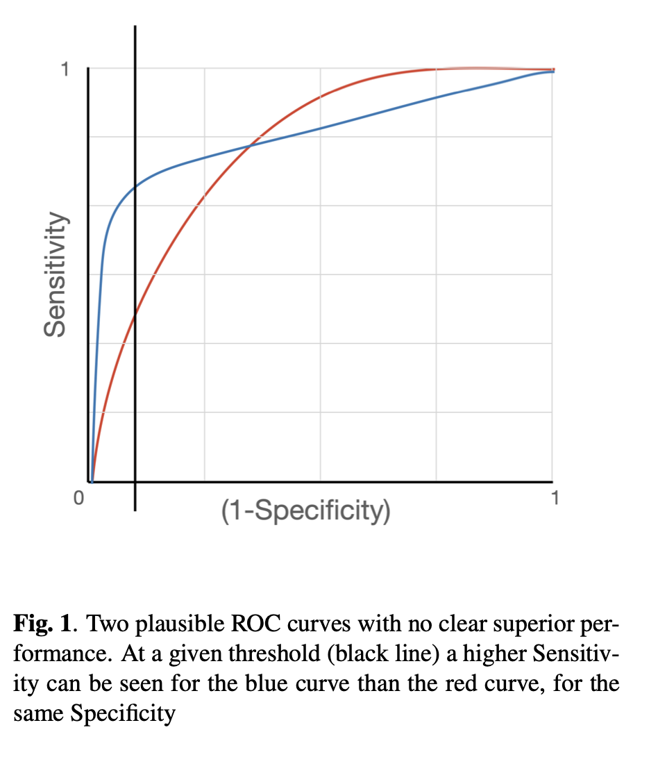
It is important to know the strengths and weaknesses of a system, and the ROC curve provides a visual indicator of whose components can be quantified, as illustrated in figure 1.
Deep learning models demonstrate outstanding performance in complex pattern recognition tasks [3] and can be applied to screening programmes where radiographs are used as a part of the screening process. If a machine learning (ML) model can perform to the standard of human readers, its integration into the cancer screening workflow can alleviate the resource burden without sacrificing performance [4]. It has been demomnstrated that in out example, Specificity is a more likely metric to anchor in this half of the Sensitivity-Specificity trade-off paradigm, and maximise Sensitivity, we can choose the benchmark Specificity of top ranking Radiologists. This way we know with reasonable certainty that the number of false positives will affect a similar proportion of people to the human system, and focus on the Sensitivity component of the metric. Evaluation is made by choosing a decision threshold such that the model’s Specificity matches with human’s Specificity, and comparing between human’s Sensitivity and model’s Sensitivity at the chosen threshold is common practice [5],andML models typically fall short of the human level Sensitivity. As such, it may be beneficial to improve the model’s performance by having an objective function that takes into account this evaluation procedure. While this can be achieved by either optimising for the AUC directly, a preferred methon may be to optimise for a model’s performance at a specific operating point. Even if the AUROC remains unchanged, the curve may be manipulated by the loss function to, in the case of the example, more accurately classify true positives at a set tru negative rate.
Optimising for AUC related metrics can be difficult as it involves ranking positive instances against negative instances in the whole population. An estimator for the AUC is the Wilcoxon Mann Whitney (WMW) statistic [6], which ranks instances in the training sample using the step function (illustreten in Figure 2). However, the WMW statistic is inappropriate as a loss function because the step function is non-differentiable. Additionally, the requirement for exhaustive ranking means that batch training with stochastic gradient descent [7] is inadequate, as it does not allow for the comparison between instances across different batches, i.e. it is non-decomposable. Previous work circumvents the non-differentiable and non-decomposable problems by using a surrogate loss that ranks instances against a threshold for the optimise Precision (the number of true positives out of all samples classified as positive) at a fixed Sensitivity[8]. This previous work can be extended upon to introduce a constrained optimisation objective that maximise Sensitivity and Specificity at a given threshold.
Examples of AUC optimisation in the past
The AUC, as a common measure for most medical imaging problems, can be formulated as a ranking problem, in which it measures the expectation of drawing positive instances that are ranked higher than negative instances using some ranking functions π : X → [0, 1]:
AUC = E(π+ > π−),
where E(.) denotes the expectation over the data distribution.
The sample estimate of the AUC is the Wilcoxon–Mann–Whitney statistic [6]:
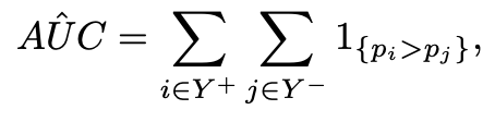
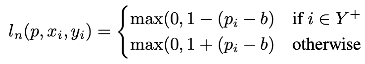
and Y +, Y − denote the positive and negative class respectively, and pi = p(xi) denotes the assessed probability, which in this case is the Machine Learning model’s output. Directly optimising for the WMW statistic is not possible given the non-differentiable nature of the step function. Previous work [9] proposed a surrogate hinge loss that acts as an upper-bound for the step function
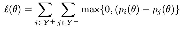
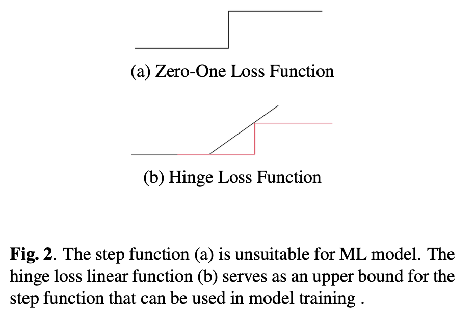
Despite the objective function being differentiable, it does not often work well in large datasets due to the non-decomposable nature of the objective, which restricts the effectiveness of batch training.
Training with Optimisation Constraints
As a way to circumvent the non-decomposable issue, [8] restricts the ranking to a threshold and optimises Sensitivity and Precision using a lower and upper bound surrogates
where b is the chosen threshold and
This formulation serves as a foundation for an adaptation of the objective function that maximises Sensitivity at a chosen Specificity.
Sensitivity@Specificity formulation
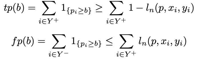
Based on the definitions of true positive (tp) and false positive (fp) in [8], their work, based on Sensitivity at a target Precision can be extended to the form relevant to the cancer screening problem outlined earlier. The Sensitivity at a set Specificity loss was derived as shown below. Sensitivity@Specificity
α : the target specificity b : the threshold at which the classification should be made
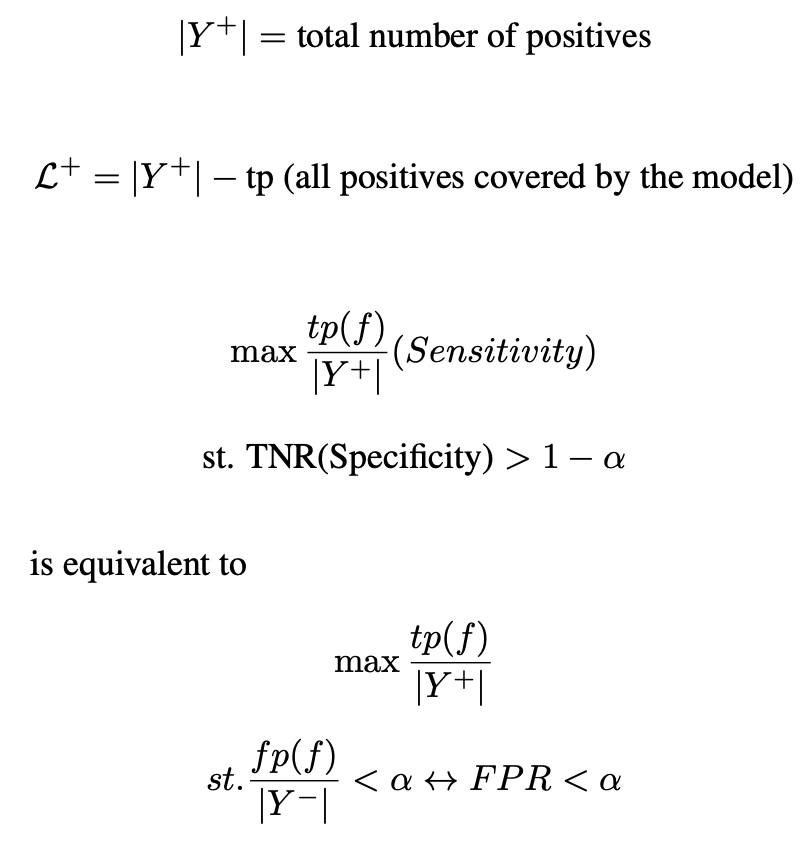
Given the previous definitions:
it is known that
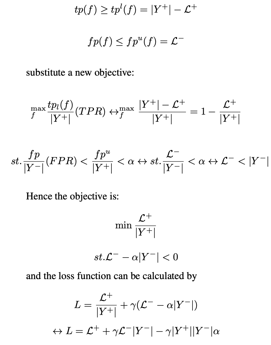
and the loss function can be calculated by
This loss function can replace BCE loss to adjust a model’s performance to achieve the objective set out in this work, maximising Sensitivity at a set Specificity.
For the Sensitivity at Specificity to work, α is the inverse of the desired Specificity, γ is a hyperparameter that requires tuning, and threshold is the threshold that is given by the post-test analysis to achieve a desired Specificity (i.e. 1-0.96=0.4 for a 96% Specificity).
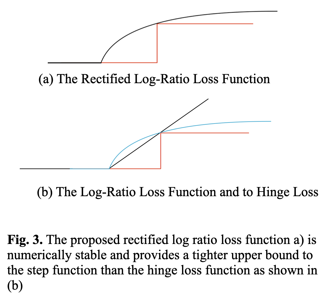
Experimental results showed the rectified linear hinge loss (as seen in Figure 2) did not improvem over cross entropy when AUROC was examined, although the Sensitivity at a target Specificity does improve. This demonstrates that the shape of the Receiver Operating Characteristic curve can be modified. In addition, the loss bound provided by a linear function can potentially be improved upon by imposing a tighter upper bound to the step function.
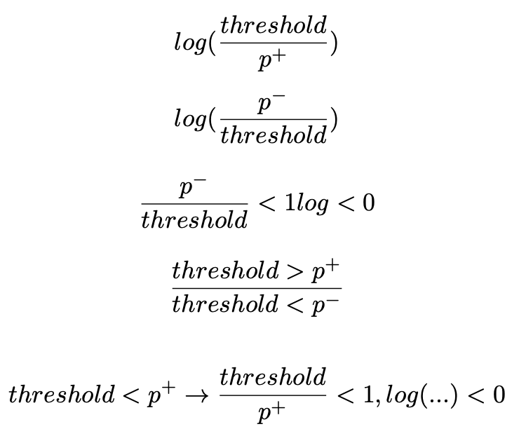
Ranking with a surrogate hinge loss is effective for maximising Sensitivity at a set Specificity, however, hinge loss does not provide a tight upper bound for the Zero-One loss step function. Cross entropy uses the log function to discriminate probabilities of groups with good performance on normally distributed datasets. The application of the log function as a tighter upper bound is an area of future work that shows theoretical promise. It has already been shown that ranking loss functions can be applied to specific non-decomposable objectives, and the work so far relies on hinge loss. Ranking with the logarithmic function as an upper bound has challenges related to numerical stability and further work to show it’s effectiveness and practical use is required. The benefits of this future work are ranking loss methods that perform as well or better than BCE loss, but can be explicitly applied to non-decomposable objectives. The formulation of a decomposable logarithmic function bounded ranking loss function is described below and illustreted in Figure 3.
Ranking loss
Binary Cross Entropy to Log Ratio
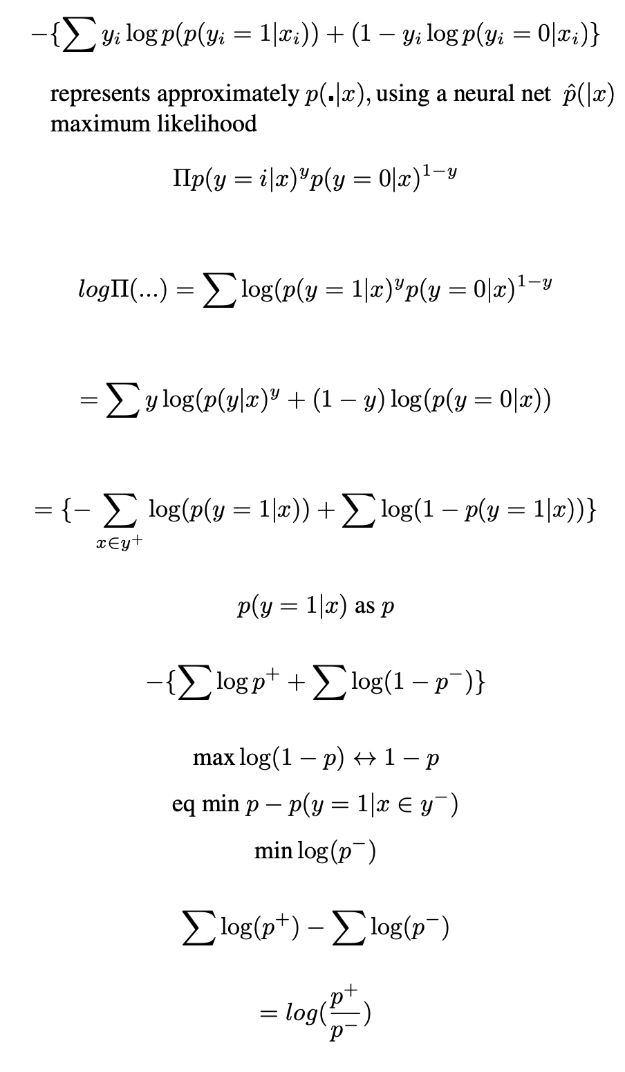
Non-Decomposable (requires a memory bank or large batch size)
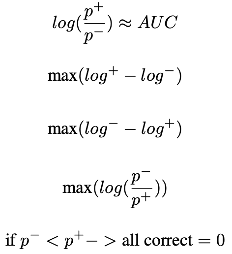
Decomposable
References
- David M. Green and John A. Swets. Signal Detection Theory and Psychophysics. New York: Wiley, 1966.
- “2016 Workforce Survey Report: AUSTRALIA”. In: Faculty of Clinical Radiology, The Royal Australian and New Zealand Collage of Radiologists®, Date of approval: 15 February 2018, 2018, pp. 44–45.
- Jeremy Irvin et al. “Chexpert: A large chest radiograph dataset with uncertainty labels and expert comparison”. In: Proceedings of the AAAI conference on artificial intelligence. Vol. 33. 01. 2019, pp. 590–597.
- Kai Qin and Hong Pan. “MDPP Technical Report, Validate and Improve Breast Cancer AI Approach”. In:(Dec. 2020).
- Mattie Salim et al. “External Evaluation of 3 Commercial Artificial Intelligence Algorithms for Independent Assessment of Screening Mammograms”. In: JAMA Oncology 6.10 (Oct. 2020), pp. 1581–1588. ISSN:2374-2437.DOI:10.1001/jamaoncol.2020.3321.eprint:https://jamanetwork.com/journals/jamaoncology/articlepdf/2769894/
jamaoncology_salim_2020_oi_200057_1619718170.78837.pdf.URL: https://doi.org/10.1001/jamaoncol.2020.3321. - H. B. Mann and D. R. Whitney. “On a Test of Whether one of Two Random Variables is Stochastically Largerthan the Other”. In: The Annals of Mathematical Statistics 18.1 (1947), pp. 50 –60. DOI: 10.1214/aoms/1177730491. URL: https://doi.org/10.1214/aoms/1177730491.
- Ian Goodfellow, Yoshua Bengio, and Aaron Courville. Deep learning. MIT press, 2016.
- Elad Eban et al. “Scalable Learning of Non-Decomposable Objectives”. In: Proceedings of the 20th International Conference on Artificial Intelligence and Statistics. Ed. by Aarti Singh and Jerry Zhu. Vol. 54. Proceedings of Machine Learning Research. PMLR, 2017, pp. 832–840.
- Lian Yan et al. “Optimizing Classifier Performance via an Approximation to the Wilcoxon-Mann-Whitney Statistic”. In: ICML. 2003.
- Mingxing Tan and Quoc Le. “EfficientNet: Rethinking Model Scaling for Convolutional Neural Networks”. In: (May 2019).
- Diederik Kingma and Jimmy Ba. “Adam: A Method for Stochastic Optimization”. In: International Conference on Learning Representations (Dec. 2014)